On backpropagation in MLP
Backpropagation based on gradient descent is the backbone of modern neural networks. However, even though the idea is simple, to explain it clearly is a bit tricky, especially when batched input is taken into consideration.
Intuition
Gradient based backpropagation is very similar to the guess a number game. When asking someone to guess a number that only we know, we can take his/her guess and compare it to our number, and tell them whether it is lower or higher. Eventually with enough iterations, he/she will arrive at a reasonable guess or even the right answer. Gradient based backpropagation is as if we compare the guess/prediction that our model gave us and tell it back whether it is higher or lower so it can adjust itself, with the right answer in this case being represented as the loss function. What is different from the guess a number game is that one: not only do we tell higher/lower, we also tell roughly how much higher/lower, and two: the input/output space is multidimensional and not a scalar, so directions are also taken into account. In fact, due to the high dimensional nature of the data space, it is quite a miracle that this simple approach even works for a lot of practical problems. At the time of this post, the theoretical justification is still quite weak as to why and how this works with random initialization in a non-convex data space full of potential local minimums and saddle points, but hey it does, just look at ChatGPT.
MLP single input
The most prevalent case of backpropagation is within a multilayer perceptron (MLP) or linear layer(s).
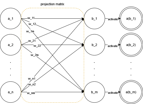
A layer in MLP is nothing but a linear projection of a vector of dimension $n$ to a vector of dimension $m$ ($n$ can equal $m$), coupled with an activation function ($a(.)$) that breaks linearity. For simplicity, the bias vector $\mathbf{b}$ is omitted here, but it may very well be seen as incorporated into the projection matrix by adding scalar $1$ as element $a_{n+1}$ in $\mathbf{a}$, resulting in the same process as described below. We define the projection matrix’s weights are our model’s parameters. Let the input vector be $\mathbf{a}$ and the output vector be $\mathbf{b}$, the following graph shows this process:
In matrix form, treating input vector as row vector (aligning with implementations of NumPy and PyTorch), we have:
\[\begin{aligned} \begin{bmatrix} a_1 & a_2 & ... & a_n \\ \end{bmatrix} \begin{bmatrix} w_{11} & w_{12} & ... & w_{1m} \\ w_{21} & w_{22} & ... & w_{2m} \\ \vdots & \vdots & \ddots & \vdots\\ w_{n1} & w_{n2} & ... & w_{nm}\\ \end{bmatrix} &= \begin{bmatrix} b_1 & b_2 & ... & b_m \end{bmatrix} \\ \text{or}, b_i &= \sum_{j=1}^n a_j \cdot w_{ji} \end{aligned}\]Now, to perform backpropagation w.r.t. the correct answer (loss function $L$), we have:
\[\begin{aligned} \frac{\partial L}{\partial \mathbf{W}} = \frac{\partial L}{\partial a(\mathbf{b})} \frac{\partial a(\mathbf{b})}{\partial \mathbf{b}} \frac{\partial \mathbf{b}}{\partial \mathbf{W}} \end{aligned}\]here $\frac{\partial L}{\partial a(\mathbf{b})}$ refers to other layers and results in a vector, $\frac{\partial a(\mathbf{b})}{\partial \mathbf{b}}$ is straightforward as we can just take the derivative of the activation function, the more troublesome part lies in $\frac{\partial \mathbf{b}}{\partial \mathbf{W}}$. Mathematically, this is finding the gradient of a matrix ($\mathbf{W}$) w.r.t. a vector ($\mathbf{b}$) and results in a 3rd order tensor in the general case. In the context of MLP, as $b_i = \sum_{j=1}^n a_j \cdot w_{ji}$, to find the gradient of $b_i$ w.r.t. an entry $w_{j’i’}$ of $\mathbf{W}$, we have:
\[\begin{aligned} \frac{\partial b_i}{\partial w_{j'i'}} &= \frac{\partial \sum_{j=1}^n a_j\cdot w_{ji}}{\partial w_{j'i'}} \\ &= \sum_{j=1}^n \delta_{jj'} \delta_{ii'} a_j & (\text{$\delta$ is the Kronecker delta}) \\ &= \delta_{ii'} a_{j'} \end{aligned}\]This eliminates the need for the 3rd dimension. For $w_{j’i’}$ where $i’$ = $i$, its derivative w.r.t. $b_i$ is $a_{j’}$, otherwise, its derivative w.r.t. $b_i$ is $0$. From the point of view of $b_i$, only $w_{j’i}$ (the i-th column) in $\mathbf{W}$ has its derivatives, and for each row $j’$ (of column $i$) the derivative is $a_{j’}$.Then, $\frac{\partial \mathbf{b}}{\partial \mathbf{W}}$ can be represented by a single matrix of the same size as $\mathbf{W}$.
Notice that $\frac{\partial L}{\partial a(\mathbf{b})} \frac{\partial a(\mathbf{b})}{\partial \mathbf{b}}$ is a vector of the same shape as $\mathbf{b}$, as typically $L$ results in a scalar and we have a scalar over vector calculus for $\frac{\partial L}{\partial a(\mathbf{b})}$ resulting in a vector of shape $\mathbf{b}$. Moreover, as $\frac{\partial a(\mathbf{b})}{\partial \mathbf{b}}$ is simply the derivative of the activation function applied elementwise on a vector of shape $\mathbf{b}$, we have a Hadamard product between two vectors of shape $\mathbf{b}$ without altering its shape.
What is interesting is that by doing the outer product $\mathbf{a}^T \cdot (\frac{\partial L}{\partial a(\mathbf{b})} \frac{\partial a(\mathbf{b})}{\partial \mathbf{b}})$, we are getting a matrix $W’$ of shape $n \times m$, the same size as the projection matrix $W$. Moreover, each entry $\mathbf{W’}_{j’i}$ of $\mathbf{W’}$ is of the following form:
\[\begin{aligned} \mathbf{W'}_{j'i} = a_{j'} \cdot (\frac{\partial L}{\partial a(\mathbf{b})} \frac{\partial a(\mathbf{b})}{\partial \mathbf{b}})_{i} && \text{($1 \le j' \le n$, $1 \le i \le m$)} \end{aligned}\]as we have justified earlier, $a_{j’}$ is indeed the derivative of the weight $W_{j’i}$ w.r.t. $b_i$. Elementwise, the equation above is none other than the result of $\frac{\partial L}{\partial a(\mathbf{b})} \frac{\partial a(\mathbf{b})}{\partial \mathbf{b}} \frac{\partial \mathbf{b}}{\partial \mathbf{W}}$, or $\frac{\partial L}{\partial \mathbf{W}}$ itself! This makes it so that the backward process is also implementable as dot product, similar to forward.
One remaining question to be answered is that we’ve only considered the case of $\frac{\partial L}{\partial a(\mathbf{b})} \frac{\partial a(\mathbf{b})}{\partial \mathbf{b}}$ for the output layer, in which case we get a vector of the same shape as the output vector. As we backpropagate through the earlier layers, this gradient vector needs to be reshaped to fit the “output layer” of the different inner layers in order for us to properly use it to calculate the gradients of the weights. It turns out that we can also simply do a dot product to solve this problem. Let $\mathbf{g} = \frac{\partial L}{\partial a(\mathbf{b})} \frac{\partial a(\mathbf{b})}{\partial \mathbf{b}}$ be the gradient vector of the outer/output layer. We can do:
\[\begin{aligned} \mathbf{g}_{prev} = \mathbf{g} \cdot \mathbf{W}^T && \text{($\mathbf{W}$ is the projection matrix of the current layer)} \end{aligned}\]where $\mathbf{g}_{prev}$ is the gradient vector for the previous layer. The justification is similar to what is shown above, as the elementwise gradient of the layer output before activation is the weights of the layer’s projection matrix.
MLP batched input
For batched input, not a lot changes except that we now have a batch of $N$ vectors as inputs and outputs. The projection matrix of the MLP model stays unchanged. We now have:
\[\begin{aligned} \begin{bmatrix} a_{11} & a_{12} & ... & a_{1n} \\ a_{21} & a_{22} & ... & a_{2n} \\ \vdots & \vdots & \ddots & \vdots\\ a_{N1} & a_{N2} & ... & a_{Nn} \\ \end{bmatrix} \begin{bmatrix} w_{11} & w_{12} & ... & w_{1m} \\ w_{21} & w_{22} & ... & w_{2m} \\ \vdots & \vdots & \ddots & \vdots\\ w_{n1} & w_{n2} & ... & w_{nm}\\ \end{bmatrix} &= \begin{bmatrix} b_{11} & b_{12} & ... & b_{1m} \\ b_{21} & b_{22} & ... & b_{2n} \\ \vdots & \vdots & \ddots & \vdots\\ b_{N1} & b_{N2} & ... & b_{Nn} \\ \end{bmatrix}\\ \text{or}, b_{bi} &= \sum_{j=1}^n a_{bj} \cdot w_{ji} \text{ ($b$ is the batch number)} \end{aligned}\]The key change here is during the outer product $\mathbf{a}^T \cdot (\frac{\partial L}{\partial a(\mathbf{b})} \frac{\partial a(\mathbf{b})}{\partial \mathbf{b}})$. Now we are no longer doing an outer product, but a full-fledged matrix multiplication between 2 matrices $\mathbf{A}^T$ and $\frac{\partial L}{\partial a(\mathbf{B})} \frac{\partial a(\mathbf{B})}{\partial \mathbf{B}}$ which can be seen as the sum of a batch of such outer products. To counter it, we need to take the average on the obtained gradients by dividing the whole by the batch size $N$ (or we can just adjust the learning rate). With modern optimizations on GPU for parallel computing, this makes the batch gradient descent based backpropagation extremely efficient to compute. Below is the (NumPy-ish) pseudocode for batch backpropagation which can be applied recursively across layers:
def layer_backpropagation(gradient, curr_output, prev_output, weights):
'''
Perform backpropagation on the current layer.

:gradients: gradients of the current layer's postactivation output w.r.t. loss
:curr_outputs: current layer's postactivation outputs (cached during forward pass)
:prev_outputs: previous layer's postactivation outputs (cached during forward pass)
:weights: weights of the current layer's projection matrix
'''
    gradient_output = gradient * derivative_activation_fn(curr_output)     # derivative_activation_fn is defined as the derivative function of the activation function
    gradient_weights = prev_output.T @ gradient_output / gradient_output.shape[0]     # x.T means transpose of x, @ means matrix multiplication
    gradient_output_prev = gradient_output @ weight.T

    return gradient_output_prev, gradient_weights
It is arguably the most important algorithm of the 21st century.