On backpropagation in CNN
Convolutional neural networks (CNN) differ from MLPs mainly for the following 2 components:
- Convolutional layer
- Pooling layer
Backpropagation in these 2 layers are a bit trickier than that of MLP.
Convolution layer
For the convolution layer, we have the following mechanism:
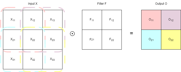
where the input $X$ ‘convolves’ with the filter $F$ to produce the output $O$. The dotted lines highlight the relevant view of $X$ w.r.t. an output square $O_k$. The backward process w.r.t. loss would then be:
\[\begin{aligned} \frac{\partial L}{\partial F} &= \frac{\partial L}{\partial O} \frac{\partial O}{\partial F} \\ \frac{\partial L}{\partial F_i} &= \sum_{k=1}^M \frac{\partial L}{\partial O_k} \frac{\partial O_k}{\partial F_i} \end{aligned}\]where $M$ is number of outputs. The summation is there because each filter is used multiple times across outputs. Then, since $\frac{\partial O_k}{\partial F_i}$ is $X_j$ from the input, where $j$ to the relevant view of $X$ is the same as $i$ to $F$, to update the gradients of the filter $F$, we have:
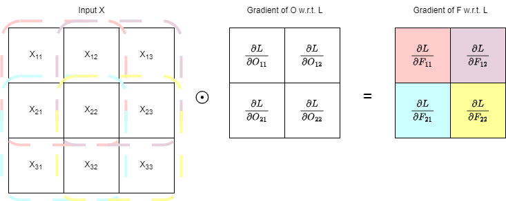
As can be seen, similar to how the backward process of MLP is also a dot product, the backward process of convolutional layer is also a convolution.
For previous layers, we also need the gradient of the input/previous layers’ output w.r.t. L. We have:
\[\begin{aligned} \frac{\partial L}{\partial X_i} = \sum_{k=1}^{M}\frac{\partial L}{\partial O_k}\frac{\partial O_k}{\partial X_i} \end{aligned}\]and in this case, $\frac{\partial O_k}{\partial X_i}$ gives us $F_j$, but $j$ to $F$ is no longer the same as $i$ to $X$. In fact, let $m$, $n$ be the height and width of $X$, $m’$, $n’$ be the height and width of $F$, then after convolution we get $O$ of height $m - m’ + 1$ and width $n - n’ + 1$. $F_{m’n’}$ participates in the creation of $O_{m-m’+1,n-n’+1}$ alongside $X_{mn}$. Notice that with regard to $O$, $m$ and $n$ of $X$ are consistent in signs while $m’$ and $n’$ of $F$ are not. This makes the $F$ rotated by 180 degrees. We then have:
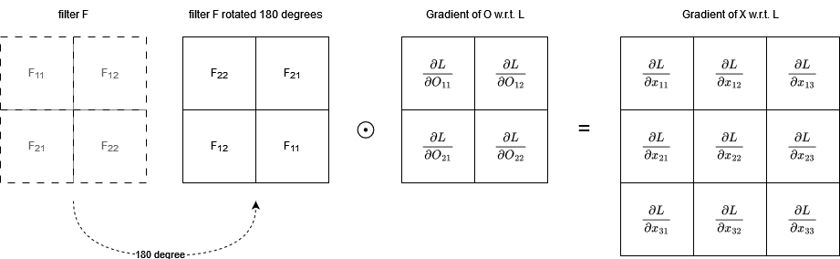
where $\odot$ is a full convolution instead of a valid convolution as above.
Pooling layer
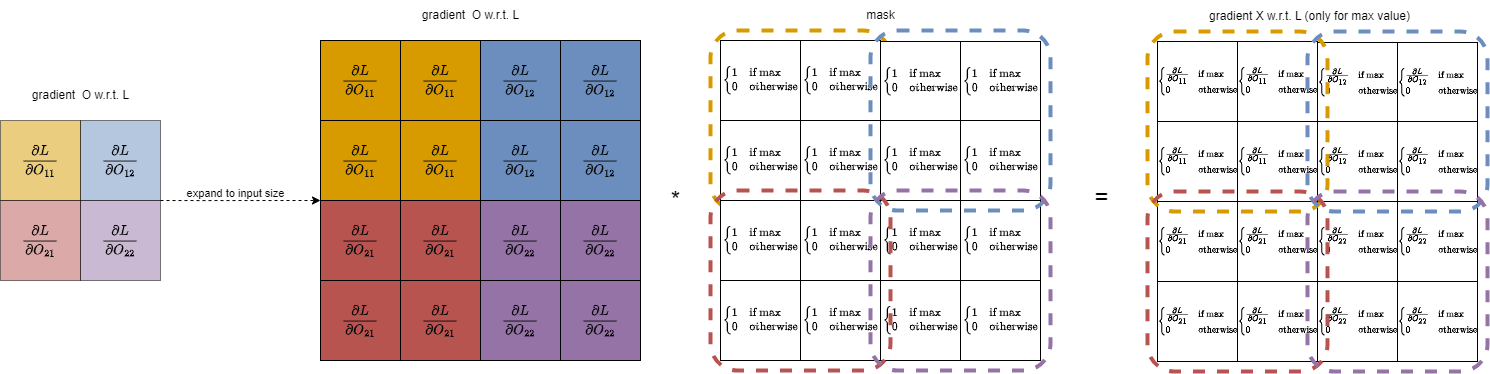
For pooling layer, we have a similar process to convolution, however we typically do not have overlapping stride, and we use the maximum instead of a weighted sum:
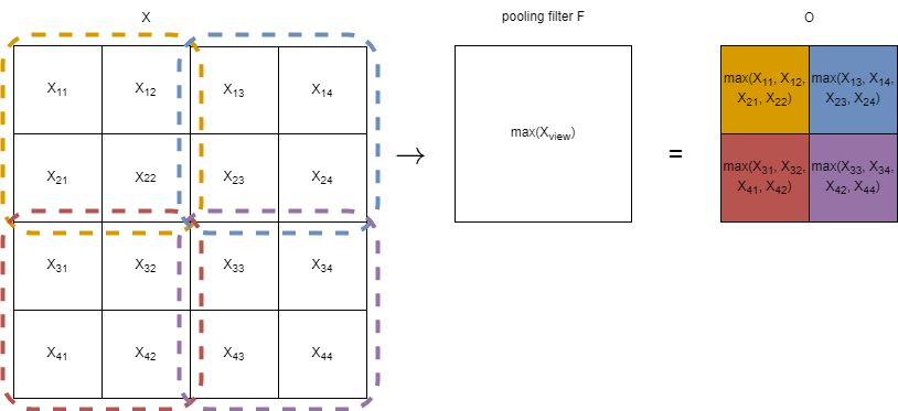
This process does not ‘alter’ the input in any way and is rather a ‘selection’. Thus, the backpropagation for the pooling layer is also a mere ‘selection’ of where to propagate the gradient back. As we only selected the maximum of the input, only the gradient of the maximum of the input w.r.t. loss should be propagated back. For implementation, we can create a binary mask indicating where are the maximum values of the input, and multiply it with the gradients of the output restored to be the size of the original input: