On KV Cache
Why This Blog?
There are many excellent resources explaining the attention mechanism and Transformer architectures. However, I’ve found that explanations of the key–value (KV) cache are often unsatisfying. More often than not, these explanations begin directly in the inference setting, without clearly connecting back to the original Transformer architecture or the underlying equations.
The goal of this blog is to bridge that gap. I aim to make an explicit connection between the canonical Transformer formulation and the practical necessity of the KV cache. By doing so, I hope to clarify why the KV cache exists, how it arises naturally from the attention mechanism, and why it is used only during autoregressive inference, and not during training.
Attention Mechanism During Training and Inference
The key to understanding the KV cache is to understand the difference between a transformer’s training and inference. I will use diagrams with fictional values to illustrate these processes.
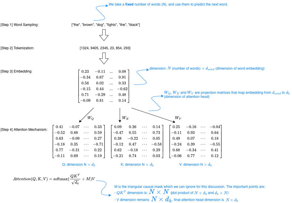
Training. The diagram below shows a hypothetical training step of a Transformer-based LLM. During training, we start with a fixed number of tokens and train the model to predict the next token. Assume our input tokens correspond to “the brown dog fights the black” (6 tokens total). As the sequence passes through the attention mechanism, it is transformed into a 6×6 attention score map, which is then used to compute a new representation for each token via weighted average.
During training, the model repeatedly samples 6 token sequences from the training corpus, and for each sample the same forward pass is performed. For example, one training instance might correspond to “the brown dog fights the black”, while the next could be “the green crocodile ate the yellow”, followed by “the white bear runs to the”, and so on. Each training sample is processed independently, and there is typically no reuse of intermediate computations across different samples.
Of course in practice, the sequence length is much larger than in this toy example, training is performed in batches, and sequences are sampled directly from large token arrays. However, the underlying idea remains the same.
Inference. When it comes to inference, even though the underlying model architecture and forward process remains the same, there is a crucial change. Instead of feeding to the model another 6 tokens, we feed the model the first token only, wait for it to generate the second token, then append it to feed the model the first and second tokens, wait for it to generate the third token, and so on. For example, we feed to the model “the”, wait for it to generates “brown”, then feed it “the brown”, wait for it to generate “dog”, then feed “the brown dog”, and so on.
This introduces a dimension of time, where we can see intuitively that there is repetition in the words “the” and “brown” at every forward step, same goes for “dog” if the generation continues. The diagram below illustrates this repetition in the forward process.
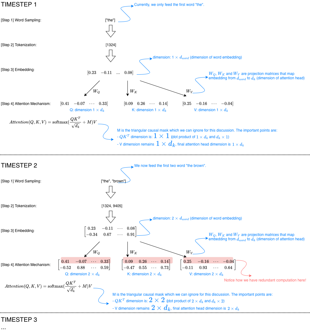
Notice how the rows corresponding to earlier timesteps (highlighted in red) are recomputed during the forward pass. A cache during inference storing the values of earlier rows should therefore be able to save computation time.
Why not Q cache?
Now, another natural question is why do we only have the KV cache, and not the Q cache? To answer this, we have to inspect closely the equation of the attention mechanism below:
\[Attention(Q, K, V) = \operatorname{softmax}(\frac{QK^T}{\sqrt{d_k}} + M)V\]First, $\operatorname{softmax}(\frac{QK^T}{\sqrt{d_k}} + M)$ is a matrix of dimension $N \times N$, where $N$ is the number of rows on $Q$ and $K$. Now, since rows of $Q$ and $K$ corresponding to earlier tokens are redundantly recomputed at each timestep, as their product, $\operatorname{softmax}(\frac{QK^T}{\sqrt{d_k}} + M)$ also contains repetitive rows which need not be calculated again. In fact, we only need to calculate the last row of $\operatorname{softmax}(\frac{QK^T}{\sqrt{d_k}} + M)$, which is the dot product between the last row of $Q$ and the entire $K^T$. Once this is done, this row is multiplied with the entirety of V to obtain the last row of the new attention head embedding.
Thus, at each timestep, we only need to compute the new row of $Q$; earlier rows of $Q$ do not need to be recomputed, as they are never used again. In contrast, the key and value matrices $K$ and $V$ are required at every timestep, which is why only they are cached during inference.