Multi-armed bandit and epsilon-greedy
Multi-armed bandit problem
A slot machine (or a one-armed bandit) has a fixed probability of winning. In a scenario where you have several slot machines, each with different winning probabilities hidden from you, how do you maximize your long term reward (profit)? This is the multi-armed bandit problem.
Exploration vs Exploitation
If the probabilities are known, the problem becomes trivial as you would just always use (exploit) the machine with the highest winning probability. However, without knowing the probabilities, you would need to first find a way to determine the probabilities yourself (explore). There is a tradeoff between exploration and exploitation as you can only choose one of the two during each time step. The former allows you to have a more accurate model of the event you are modeling, while the latter allows you to best utilize your existing model to maximize rewards. This is a central theme in reinforcement learning.
Epsilon-greedy algorithm
The epsilon-greedy algorithm is a straightforward way of handling the above. The key idea is to almost always exploit the machine with the highest winning probability based on historical experience (which may be inaccurate and differ from true probabilities), but once in a while to use a random machine. This allows us to adjust the historical experience to make it more accurate. The probability of exploring a random machine is $\epsilon$, while the probability of exploiting the winningest machine is $1 - \epsilon$.
How to determine the probabilities
To determine the probabilities, we simply need to average the historical reward data. By the law of big numbers, an infinite amount of samples will lead our estimate to converge to the true probabilities. Let’s formally define the above problem in mathematical terms: let $t$ denote a timestep, let $A_t$ denote an action at timestep $t$ (in this setting, an action is to use a particular machine), $R_t$ denote a reward at timestep $t$ (in this setting, a reward is either hitting the jackpot or fail to hit the jackpot), let $Q_t(a)$ be our estimate of the reward at timestep $t$ by performing action $a$. At any given time, there will be a true reward $Q^*_t(a) = \mathbb{E}[R_t \vert A_t = a]$, and we estimate the former using $Q_t(a)$ with limited historical data:
\[\begin{aligned} Q_t(a) = \frac{\text{sum of rewards when } a \text{ taken prior to } t}{\text{number of times } a \text{ taken prior to } t} = \frac{\sum_{i=1}^{t-1} R_i \cdot \mathbb{1}_{A_i=a}}{\sum_{i=1}^{t-1} \mathbb{1}_{A_i=a}} \end{aligned}\]where $\mathbb{1}_{predicate}$ is 1 if predicate is true and 0 otherwise.
To calculate the above average, it is unnecessary to keep all past values in memory during each timestep as we have the following recurrence relation:
\[\begin{aligned} Q_{n+1} &= \frac{1}{n}\sum_{i=1}^{n}R_i\\ &= \frac{1}{n} (R_n + \sum_{i=1}^{n-1}R_i)\\ &= \frac{1}{n} (R_n + (n-1)\frac{1}{n-1}\sum_{i=1}^{n-1}R_i)\\ &= \frac{1}{n} (R_n + (n-1)Q_n)\\ &= \frac{1}{n} (R_n + nQ_n - Q_n)\\ &= Q_n + \frac{1}{n}[R_n - Q_n] \end{aligned}\]This effectively reduces both the time and memory complexity from $O(n)$ to $O(1)$ during each time step.
What about non-stationary distribution?
The above formula works well when the slot machines’ distributions are stationary. However, if the underlying distributions change over time, then past results may not accurately reflect the current distribution, and we should assign more weights to the more current results. This can be elegantly done by changing slightly the above formula:
\[\begin{aligned} Q_{n+1} &= Q_n + \alpha[R_n - Q_n] \end{aligned}\]Where $\alpha \in (0, 1]$ is constant and controls how much more weight do we assign to current results compared to historical results. When $\alpha = 1$, we effectively have the moving average described above. For each time step, the weight decay can be shown as follow:
\[\begin{aligned} Q_n + \alpha[R_n - Q_n] &= \alpha R_n + (1 - \alpha)Q_n\\ &= \alpha R_n + (1 - \alpha)[\alpha R_{n-1} + (1-\alpha) Q_{n-1}]\\ &= \alpha R_n + (1 - \alpha)\alpha R_{n-1} + (1 - \alpha)^2 \alpha R_{n-2} + ... + (1 - \alpha)^{n-1}\alpha R_1 + (1 - \alpha)^n Q_1\\ &= (1 - \alpha)^n Q_1 + \sum_{i=1}^{n}\alpha (1 - \alpha)^{n-i}R_i \end{aligned}\]It can be shown that the sum of the weights in the above equation equals 1:
\[\begin{aligned} (1 - \alpha)^n + \sum_{i=1}^{n}\alpha (1 - \alpha)^{n-i} &= (1-\alpha)^n + \alpha(1-\alpha)^n \sum_{i=1}^n (1-\alpha)^{-i} \\ &= (1 - \alpha)^n (1 + \alpha \sum_{i=1}^n (1 - \alpha)^{-i}) \end{aligned}\]Notice the geometric series $ \sum_{i=1}^n (1 - \alpha)^{-i}$ which can be simplified using the formula $S_n = \frac{a_1 (1 - r^n)}{1 - r}$ where $a_1$ is the first term, $r$ is the common ratio and $n$ is the number of terms. We can simplify as follow:
\[\begin{aligned} (1 - \alpha)^n (1 + \alpha \sum_{i=1}^n (1 - \alpha)^{-i}) &= (1 - \alpha)^n (1 + \alpha (\frac{(1 - \alpha)^{-1}(1 - (1 - \alpha)^{-n})}{1 - (1 - \alpha)^{-1}})) \\ &= (1 - \alpha)^n (1 + \alpha (\frac{(1 - \alpha)^{-1} - (1 - \alpha)^{-1}(1 - \alpha)^{-n}}{1 - (1 - \alpha)^{-1}}))\\ &= (1 - \alpha)^n (1 + \alpha (\frac{(1 - \alpha)^{-1} - (1 - \alpha)^{-1}(1 - \alpha)^{-n}}{\frac{1 - \alpha}{1 - \alpha} - \frac{1}{1 - \alpha}}))\\ &= (1 - \alpha)^n (1 + \alpha (\frac{(1 - \alpha)^{-1} - (1 - \alpha)^{-1}(1 - \alpha)^{-n}}{-\alpha(1-\alpha)^{-1}}))\\ &= (1 - \alpha)^n (1 + \alpha (\frac{-1 + (1 - \alpha)^{-n}}{\alpha}))\\ &= (1 - \alpha)^n (1 - 1 + (1-\alpha)^{-n})\\ &= 1 \end{aligned}\]As the weights sum to 1 and weights decay exponentially through time, this is also called an exponential recency-weighted average.
Implementation
Below is the key implementation part for the epsilon-greedy:
  # Q_arr is the current estimates of the arms
  # N_arr is the number of times each action is taken
  # bandit is the multibandit model
  for time_step in range(num_time_step):
    A_star = np.random.choice(np.where(Q_arr == max(Q_arr))[0]) # exploitation, break tie randomly
    A_random = np.random.choice(actions) # exploration
    A = np.random.choice([A_random, A_star], p=[epsilon,  1 - epsilon]) # explore with probability epsilon, else exploit
    curr_R = bandit.sample(A) # get current reward
    N_arr[A] = N_arr[A] + 1

    if alpha == None:
      # incremental averaging
      Q_arr[A] = Q_arr[A] + (1 / N_arr[A]) * (curr_R - Q_arr[A])
    else:
      # recency-weighted averaging
      Q_arr[A] = Q_arr[A] + alpha * (curr_R - Q_arr[A])

    R_over_t.append(curr_R) # cumulative rewards
Some experimentation results on a 3-armed problem can be seen here:
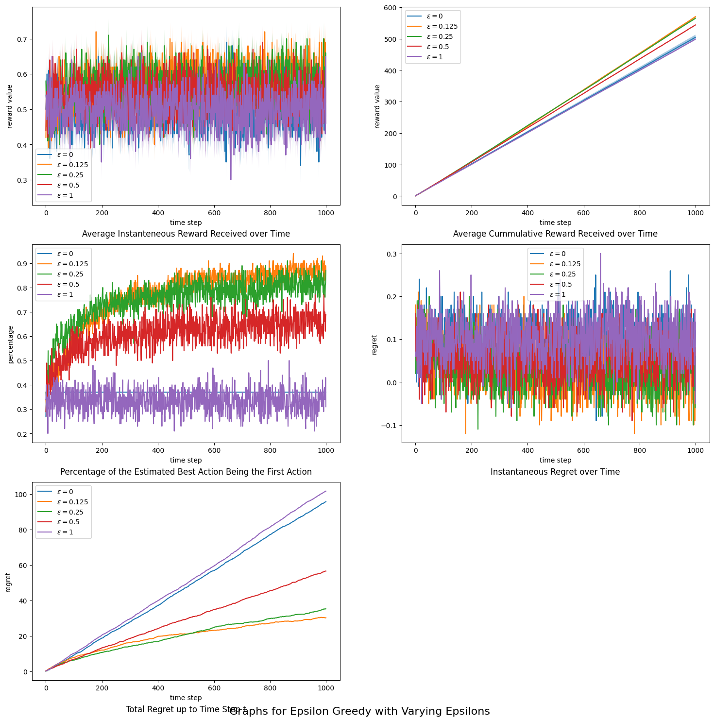
We can conclude that the value of $\epsilon$ does affect convergence, and a small value works best in the long run.
Reference: Reinforcement Learning - An Introduction by Richard S. Sutton and Andrew G. Barto (chapter 2)