Bellman equation, SARSA and Q-learning
Finite Markov decision processes
It is necessary to first establish a key concept - finite Markov decision processes (MDPs), as it is the classical formulation of the problem space comprising of most of reinforcement learning. MDPs comprise of states (S), actions (A) and rewards (R), where states can be changed by taking actions, and each action has an associated reward. In fact, the idea is quite intuitive and the following figure should be enough to give you a very good idea of MDP:
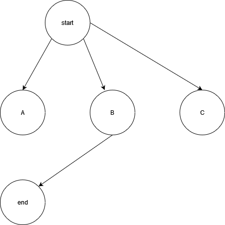
The circles are states, the arrows are actions, and each action has an associated reward (not shown in graph). There is no limitation on how many states or what states are connected, states can connect to themselves and arrows can also be both ways. Mathematically, MDP is a probabilistic model of all the possible actions and their consequences for an event. Of course, we typically do not have such a model, but envisioning such a model can facilitate our theoretical analysis for a lot of problems.
Bellman equation
Say we have a finite MDP (which means the total number of states are finite), and we want to maximize the total reward during an episode, where an episode comprises of all the steps we take from a start state till an end state. Without knowing the structure of the MDP and starting from a random state, this state space search is a key objective of reinforcement learning. To define the above formally, let $t$ be a timestep and $R_{t+1}$, $R_{t+2}$, $R_{t+3}$, … be rewards received after timesteps $t$, $t+1$, $t+2$, …, then we need to maximize the expected return denoted by $G_t$, where $G_t = R_{t+1} + R_{t+2} + … + R_{T}$, where $T$ is the final time step. Sometimes, there is no end to the process and we can’t define an episode, then $G_t$ can still be defined as follow: $G_t = \gamma R_{t+1} + \gamma^2 R_{t+2} + … = \sum_{k=0}^{\infty}\gamma^k R_{t+k+1}$. $\gamma$ here is the discount factor as mentioned by the previous post, it assigns more weight to more immediate rewards. Note that even though this is a sum of an infinite number of terms, as long as $0 \le \gamma < 1$ and the rewards $R_{t+1}, R_{t+2}, …$ are bounded by a finite number, we can still find a closed-form solution to the sum. For example, if all rewards are $1$, then we have $G_t = \sum_{k=0}^{\infty}\gamma^k = \frac{1}{1-\gamma}$.
A very important property of the expected return is its ability to be defined recursively as so:
\[\begin{aligned} G_t &= R_{t+1} + \gamma R_{t+2} + \gamma^2 R_{t+3} + ...\\ &= R_{t+1} + \gamma(R_{t+2} + \gamma R_{t+3} + ...)\\ &= R_{t+1} + \gamma G_{t+1} \end{aligned}\]As we will see, this recursion allows us to incrementally extract information about the MDP throughout our episode (if we have one), which is a key idea of the temporal difference learning algorithms presented below.
Now, we can continue to formally define our objective functions about the reward. We can define in two ways: value function ($v_\pi (s)$) which is from the perspective of a state (s), and action value function ($q_\pi (s, a)$) which is from the perspective of a state (s) and a chosen action (a). The two are in fact equivalent (as they describe the same phenomenon) and are bounded by the following relationship: $v_\pi (s) = \sum_a q_\pi (s, a)$. $\pi$ here is a policy function which determines what action to take during the process, the epsilon-greedy mentioned in the previous post is an example of policy. In stochastic models, $\pi(a \vert s)$ signifies the probability of taking action $a$ at state $s$ following policy $\pi$. The formal definitions are:
\[\begin{aligned} v_\pi (s) \dot{=} \mathbb{E}_\pi [G_t | S_t = s] = \mathbb{E}_\pi [\sum_{k=0}^\infty \gamma^k R_{t + k + 1} | S_t = s] \end{aligned}\] \[\begin{aligned} q_\pi (s, a) \dot{=} \mathbb{E}_\pi [G_t | S_t = s, A_t = a] = \mathbb{E}_\pi [\sum_{k=0}^\infty \gamma^k R_{t + k + 1} | S_t = s, A_t = a] \end{aligned}\]where $\dot{=}$ is the symbol for definition, $\mathbb{E}_\pi[.]$ denotes the expected value of a random variable given the agent follows policy $\pi$, in the case of MDP, it is the expected value of future rewards, and $t$ is any time step. Note that the expected value is only needed if we have a stochastic action space, where each action is not deterministic but a probability under $\pi$, otherwise, we wouldn’t need it.
Now, using the recursive property of the expected return as mentioned above, we can further develop the equations into:
\[\begin{aligned} v_\pi(s) &\dot{=} \mathbb{E}_\pi[G_t | S_t = s] \\ &= \mathbb{E}_\pi [R_{t+1} + \gamma G_{t+1} | S_t = s]\\ &= \sum_a \pi(a|s) \sum_{s'}\sum_r p(s', r|s, a)[r + \gamma \mathbb{E}_\pi[G_{t+1} | S_{t+1} = s']]\\ &= \sum_a \pi(a|s) \sum_{s', r} p(s', r|s, a)[r + \gamma v_\pi(s')] \end{aligned}\] \[\begin{aligned} q_\pi(s, a) &\dot{=} \mathbb{E}_\pi[G_t | S_t = s, A_t = a] \\ &= \mathbb{E}_\pi [R_{t+1} + \gamma G_{t+1} | S_t = s, A_t = a]\\ &= \sum_{s'}\sum_r p(s', r|s, a)[r + \gamma (\sum_{a'} \pi(a'|s') \mathbb{E}_\pi[G_{t+1} | S_{t+1} = s', A_{t+1} = a'])]\\ &= \sum_{s', r} p(s', r|s, a)[r + \gamma (\sum_{a'} \pi(a'|s') q_\pi(s', a'))] \end{aligned}\]where $s’$ is the next state obtained after the chosen action $a$, $r$ is the associated reward, and $a’$ are the actions available at state $s’$. This is the Bellman equation (defined in terms of state and state-action). It formally breaks the objective function into a tangible part which we can compute at a given timestep and a recursion to be computed in the next timesteps. Temporal difference algorithms presented below highlight this idea.
Q-learning and SARSA
Q-learning is an algorithm that optimizes the action-value equation $q^*(s, a)$ that is the solution to the Bellman optimality equation, which is the maximal solution to the Bellman equation under an optimal policy $\pi^*$. Say we have a MDP and we randomly initialized its action value function, except the terminal state where we have Q(terminal, .) = 0. We can then use the Q-learning algorithm to update its function value:
parameters: $\alpha \in (0, 1]$, small $\epsilon$ > 0, $\gamma \in [0, 1)$
loop for each episode:
$\quad$Initialize $S$ (randomly except Q(terminal, .) = 0)
$\quad$Loop for each step of episode:
$\qquad$Choose $A$ from $S$ using some policy derived from $Q$ (eg $\epsilon$-greedy)
$\qquad$Take action $A$, observe $R, S’$
$\qquad Q(S,A) \leftarrow Q(S,A) + \alpha[R+\gamma \max_a Q(S’, a) - Q(S, A)]$
$\qquad S \leftarrow S’$
$\quad$ until $S$ is terminal
Notice how in the update step for the action-value function $Q$, we use $\max_a(S’, a)$ to choose the next action independent of the policy $\pi$ ($\epsilon$-greedy in this case). This is thus called an off-policy algorithm.
A similar algorithm SARSA (derived from ($S_t, A_t, R_{t+1}, S_{t+1}, A_{t+1}$) at each iteration) slightly modifies the above algorithm to instead follow the existing policy:
parameters: $\alpha \in (0, 1]$, small $\epsilon$ > 0, $\gamma \in [0, 1)$
loop for each episode:
$\quad$Initialize $S$ (randomly except Q(terminal, .) = 0)
$\quad$Loop for each step of episode:
$\qquad$Choose $A$ from $S$ using some policy derived from $Q$ (eg $\epsilon$-greedy)
$\qquad$Take action $A$, observe $R, S’$
$\qquad$Choose $A’$ from $S’$ using policy derived from $Q$ (eg $\epsilon$-greedy) $\qquad Q(S,A) \leftarrow Q(S,A) + \alpha[R+\gamma Q(S’, A’) - Q(S, A)]$
$\qquad S \leftarrow S’; A \leftarrow A’$
$\quad$ until $S$ is terminal
This algorithm chooses the next action $A’$ based on the policy $\pi$ and is thus called an on-policy algorithm. Due to that, it no longer directly optimizes the Bellman optimal equation, but something close. As a result, Q-learning can sometimes lead to more optimal solutions (lower bias) but has higher instability and variance during training. SARSA on the other hand is more conservative during training (as it uses the policy it learned to avoid potential high penalties), thus results in lower variance but higher bias.
Both Q-learning and SARSA are proven to converge under certain conditions easily met in practice. However a common condition for convergence proof is to be able to visit all states infinitely many times. This is sometimes challenging or impossible to meet in practice. The proof of convergence is quite technical but I found some papers regarding it: convergence for SARSA, convergence for Q-learning. Read if you like to be tortured ![]() .
.
Implementation of QLearning
We use the openai gymnasium to implement the algorithm. Gynmasium offers a standard environment to approximate the underlying MDP. In particular, we use the pre-built Taxi environment, which is a toy environment in which the agent (a taxi driver) learns how to navigate the map to pickup and drop customers.
The full code is adapted from an excellent tutorial here with minor adjustments:
import gymnasium as gym
import numpy as np
import random
from tqdm import tqdm
from gymnasium.wrappers import RecordVideo

def main():
    env = gym.make('Taxi-v3')
    state = env.reset()
    state_size = env.observation_space.n
    action_size = env.action_space.n
    qtable = np.zeros((state_size, action_size)) # memory for action-value function

    learning_rate = 0.9 # alpha
    discount_rate = 0.8 # gamma
    epsilon = 1.0
    decay_rate = 0.005 # gradually decrease epsilon over time

    num_episodes = 1000
    max_steps = 99

    # TRAINING
    for episode in tqdm(range(num_episodes)):
        state = env.reset()[0]
        terminated, truncated = False, False

        for s in range(max_steps):
            if random.uniform(0, 1) < epsilon:
                action = env.action_space.sample()

            else:
                action = np.argmax(qtable[state, :])

            new_state, reward, terminated, truncated, info = env.step(action)
            # Q(S,A) ← Q(S,A) + α[R+ γ*max_aQ(S′,a) − Q(S,A)]
            qtable[state, action] = qtable[state, action] + learning_rate * (reward + discount_rate * np.max(qtable[new_state, :]) - qtable[state, action])
            state = new_state

            if terminated or truncated: break

        epsilon = np.exp(-decay_rate * episode)
    env.close()
    print(f"training completed over {num_episodes} episodes")

    # EVALUATING
    base_env = gym.make('Taxi-v3', render_mode='rgb_array')
    env = RecordVideo(base_env, video_folder="./videos", disable_logger=True)

    state = env.reset()[0]
    terminated, truncated = False, False
    rewards = 0

    for s in range(max_steps):
        action = np.argmax(qtable[state, :]) # purely greedy as we have a trained agent
        new_state, reward, terminated, truncated, info = env.step(action)
        rewards += reward
        print(f"score at step {s}: {rewards}")
        state = new_state
        if terminated or truncated: break
    env.close()

if __name__ ==  "__main__":
    main()
After 1000 episodes of training, we do have a reasonable taxi driver who is not drunk and not lost:
Reference: Reinforcement Learning - An Introduction by Richard S. Sutton and Andrew G. Barto (chapters 3 and 6)