Policy gradient algorithms
Problem with tabular reinforcement learning techniques
Methods such as SARSA and Q-learning presented in the previous post involve an action-value function from which we can generate a policy. The action-value function can be tabular, in which case it suffers from the curse of dimensionality and becomes infeasible for large or continuous state spaces, or it can be approximated by a function approximator such as a neural network or a decision tree, in which case it is prone to be unstable.
If we look at the optimization through another angle, we can simply approximate the policy function directly. By extracting observations of the state as features and ouputting an associated value, we can generate a stochastic representation of the policy function $\pi(a|s)$ and adjust it using gradient based methods.
Evaluating policy
Again, we need a way to evaluate the effectiveness of policies that we create. Optimally, we can define a reward function as so:
\[J(\theta) = \sum_{s\in S}d^\pi(s)V^\pi(s) = \sum_{s\in S}d^\pi(s)\sum_{a\in A}\pi_\theta(a|s)Q^\pi(s, a)\]where $s$ are states, $a$ are actions, $\pi$ is our policy parameterized by $\theta$, and $d^\pi(s)$ is the stationary distribution of a state $s\in S$ under the policy $\pi$. Stationary distributions are long-term distributions of a dynamic equilibrium attained in a Markov decision process when time tends to infinity, or $d^\pi(s) = \lim_{t\rightarrow\infty}P(s_t = s | s_{start}, \pi_\theta)$. When the underlying MDP is ergodic, this distribution does not depend on the starting point $s_{start}$ and only depends on the policy $\pi_\theta$.
However, as generally the underlying environment or MDP is unknown, the stationary distribution is intractable. It is therefore more practical to define $J(\theta)$ for an episodic event:
\[\begin{aligned} J(\theta) = V_{\pi_\theta}(s_0) \end{aligned}\]Where $V_{\pi_\theta}$ is the true value function for policy $\pi_\theta$, and $s_0$ is a starting state. Even optimizing $V_{\pi_\theta}(s_0)$ seems to be a challenging task, as despite starting from a fixed starting state $s_0$, there is a hidden stationary distribution of state visit likelihood that depends on $\theta$ and that affects the value function. However, a very nice theoretical result presented next allows us to settle this problem.
Policy Gradient Theorem
This section is pretty dense. I will shamelessly copy the proof on Lilian Weng’s excellent blog about this topic, but I will add a bit more explanation and modify here and there to some key steps which I find important.
First, we start with the gradient of the value function, pay attention to the red part:
\[\begin{aligned} \nabla_\theta V^\pi(s) &= \nabla_\theta(\sum_{a\in A}\pi_\theta(a|s)Q^\pi(s,a))\\ &= \sum_{a\in A}(\nabla_\theta \pi_\theta(a|s)Q^\pi(s,a) + \pi_\theta(a|s)\color{red}{\nabla_\theta Q^\pi(s,a)}) & \text{; product rule} \\ &= \sum_{a\in A}(\nabla_\theta \pi_\theta(a|s)Q^\pi(s,a) + \pi_\theta(a|s) \color{red}{\nabla_\theta \sum_{s', r}P(s', r|s,a)(r+V^\pi(s'))}) & \text{; s' are next states following action a}\\ &= \sum_{a\in A}(\nabla_\theta \pi_\theta(a|s)Q^\pi(s,a) + \pi_\theta(a|s) \color{red}{\sum_{s', r}P(s',r|s,a)\nabla_\theta V^\pi(s')}) & \text{;$P(s',r|s,a)$ and $r$ not a function of $\theta$}\\ &= \sum_{a\in A}(\nabla_\theta \pi_\theta(a|s)Q^\pi(s,a) + \pi_\theta(a|s) \color{red}{\sum_{s'}P(s'|s,a)\nabla_\theta V^\pi(s')}) & \text{;$P(s'|s,a) = \sum_r P(s', r|s,a)$}\\ &= \sum_{a\in A}(\nabla_\theta \pi_\theta(a|s)Q^\pi(s,a) + \pi_\theta(a|s) \sum_{s'}P(s'|s,a)\color{orange}{\nabla_\theta V^\pi(s')}) \end{aligned}\]Notice how the orange part is a recurrence relation. This is the first key to what we are going to do. Before going further, let’s define $p^\pi(s\rightarrow s’, k)$ as the probability of transitioning from state $s$ to state $s’$ in $k$ timesteps following policy $\pi$. Then, it should be easy to see that:
\[\begin{aligned} p^\pi(s \rightarrow s, 0) &= 1 & \\ p^\pi(s \rightarrow s', 1) &= \sum_a \pi_\theta(a|s)P(s'|s,a) \\ p^\pi(s \rightarrow s'', 2) &= \sum_{s'}p^\pi(s \rightarrow s', 1) p^\pi(s' \rightarrow s'', 1) \\ p^\pi(s \rightarrow s''', 3) &= \sum_{s''}p^\pi(s \rightarrow s'', 2) p^\pi(s'' \rightarrow s''', 1) \\ .\\ .\\ .\\ p^\pi(s \rightarrow s^{(k+1)}, k+1) &= \sum_{s^{(k)}} p^\pi(s \rightarrow s^{(k)}, k) p^\pi(s^{(k)} \rightarrow s^{(k+1)}, 1) \end{aligned}\]Continuing our initial derivation above, and let $\phi(s) = \sum_{a\in A}\nabla_\theta \pi_\theta(a|s)Q^\pi(s,a)$ to simplify writing, we have:
\[\begin{aligned} \nabla_\theta V^\pi(s) &= \sum_{a\in A}(\nabla_\theta \pi_\theta(a|s)Q^\pi(s,a) + \pi_\theta(a|s) \sum_{s'}P(s'|s,a)\color{orange}{\nabla_\theta V^\pi(s')}) \\ &= \phi(s) + \sum_{a\in A}\pi_\theta(a|s) \sum_{s'}P(s'|s,a)\color{orange}{\nabla_\theta V^\pi(s')} \\ &= \phi(s) + \sum_{s'} \sum_{a} \pi_\theta(a|s) P(s'|s, a)\color{orange}{\nabla_\theta V^\pi(s')} \\ &= \phi(s) + \sum_{s'} p^\pi(s \rightarrow s', 1)\color{orange}{\nabla_\theta V^\pi(s')}\\ &= \phi(s) + \sum_{s'} p^\pi(s \rightarrow s', 1)\color{orange}{[\phi(s') + \sum_{s''}p^\pi(s'\rightarrow s'', 1)\nabla_\theta V^\pi(s'')]}\\ &= \phi(s) + \sum_{s'} p^\pi(s \rightarrow s', 1)\phi(s') + \sum_{s''}p^\pi(s \rightarrow s'', 2)\color{purple}{\nabla_\theta V^\pi(s'')}\\ &= \phi(s) + \sum_{s'} p^\pi(s \rightarrow s', 1)\phi(s') + \sum_{s''}p^\pi(s \rightarrow s'', 2)\color{purple}{[\phi(s'') + \sum_{s'''}p^\pi(s'' \rightarrow s''', 1)\nabla_\theta V^\pi(s''')]}\\ &= \phi(s) + \sum_{s'} p^\pi(s \rightarrow s', 1)\phi(s') + \sum_{s''}p^\pi(s \rightarrow s'', 2)\phi(s'') + \sum_{s'''}p^\pi(s \rightarrow s''', 3)\color{pink}{\nabla_\theta V^\pi(s^{(4)})} \\ &= ... \text{ ;keep unrolling the gradient}\\ &= \underbrace{\sum_{x\in S}\sum_{k=0}^\infty}_{\text{general case}} p^\pi(s\rightarrow x, k)\phi(x) \end{aligned}\]It should be noted that $\sum_{x\in S}\sum_{k=0}^\infty$ is the general case under the assumption that all states can be visited an infinite amount of times from a starting state $s$. In practice, we may only have a finite number of visits on a subset of states.
Now, notice how $p^\pi(s\rightarrow x, k)$ attains a dynamic equilibrium in a Markov decision process and becomes a stationary distribution as time goes to infinity ($\lim_{k\rightarrow \infty}p^\pi(s\rightarrow x, k) = \text{const}$). This is exactly how Google’s page-rank works, and is the second key to our proof. Starting from a random state $s_0$, let $\eta (s) = \sum_{k=0}^\infty p^\pi(s_0\rightarrow s, k)$, which can be thought of as some kind of likelihood to visit state $s$ starting from state $s_0$ over an infinite horizon (available because of the stability over time mentioned above), we have:
\[\begin{aligned} \nabla_\theta J(\theta) &= \nabla_\theta V^\pi(s_0) \\ &= \sum_{s}\sum_{k=0}^\infty p^\pi(s_0\rightarrow s, k)\phi(s)\\ &= \sum_{s} \eta(s) \phi(s) & \text{;here $\eta(s)$ depends on $\pi_\theta$, and serves as some kind of weight}\\ &\propto \sum_{s}\frac{\eta(s)}{\sum_{s}\eta(s)}\phi(s) & \text{;Normalize $\eta(s)$ to be a probability distribution, capturing weight information}\\ &= \sum_s d^\pi(s) \sum_a \nabla_\theta \pi_\theta(a|s)Q^\pi(s, a) & \text{;$d^\pi(s) = \frac{\eta(s)}{\sum_{s}\eta(s)}$ is a stationary distribution} \\ &= \sum_s d^\pi(s) \sum_a \pi_\theta(a|s)Q^\pi(s, a)\frac{\nabla_\theta \pi_\theta(a|s)}{\pi_\theta(a|s)}\\ &= \mathbb{E}_\pi[Q^\pi(s, a)\nabla_\theta \ln \pi_\theta(a|s)] & \text{;Because $(\ln \pi_\theta(a|s))' = \frac{1}{\pi_\theta(a|s)}$} \end{aligned}\]Where $\mathbb{E}_\pi$ refers to $\mathbb{E}_{s\sim d_\pi, a \sim \pi}$ when both state and action distributions follow the policy $\pi_\theta$ (on policy). What is important to note here is that despite taking the gradient over $V_{\pi_\theta}$, we end up not taking the gradient over the hidden state distribution $d_\pi$ which is intractable, but only over the immediate policy distribution $\pi$. Moreover, $d_\pi$ can be sampled through experience as we don’t use its gradient but itself.
The policy gradient theorem is an important result that lays the theoretical foundation for various optimization algorithms.
REINFORCE (direct implementation of policy gradient theorem)
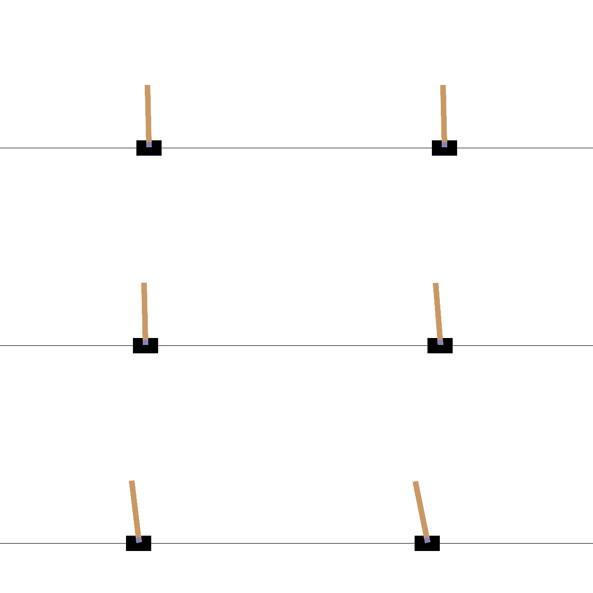
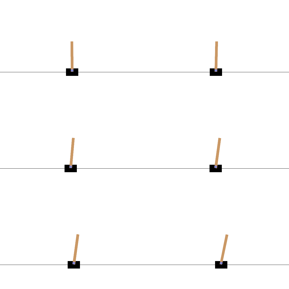
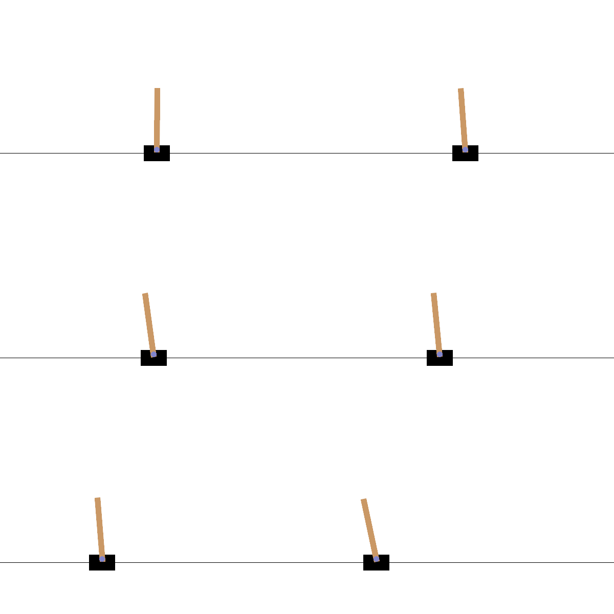
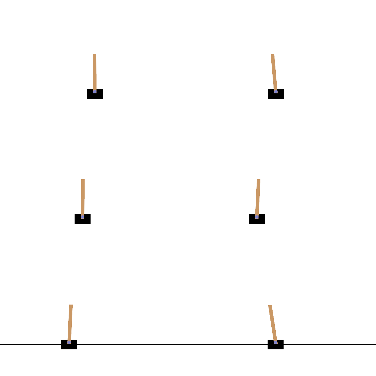
REINFORCE algorithm is a direct implementation of the result of policy gradient theorem above. Pytorch has a nice implementation here which I will break down. First, let’s define the environment and the problem of this example here, where we have a pole attached to a cart by an un-actuated joint. Un-actuated basically means the joint is not fixed and the pole can rotate freely. Our goal is to stabilize the pole such that its end opposite to the joint stays on top of the cart and does not fall down. We do so using 2 actions: 1. pushing the cart left by a fixed force 2. pushing the cart right by a fixed force. The observations we can get following each action can be defined using a 4 tuple: (cart position, cart velocity, pole angle, pole angular velocity). When the cart leaves the (-2.4, 2.4) range or when the pole angle leaves the (-0.2095rad, 0.2095rad) range, we consider the pole to be no longer stabilized and the episode ends. As our goal is to stabilize the pole, for each time step we add a reward of +1. The default reward threshold is set to 475, which can be approximately thought of as if we are able to get to 475 time steps without the pole falling, we consider to have a good policy to stabilize the pole. We can simply do gym.make('CartPole-v1') to initialize this environment using OpenAI’s gynmasium library.
Now, as we are doing policy gradient, we need a function to define our policy. In Pytorch’s code, this is done using a simple feedforward neural network with 1 hidden layer of dimension 128:
class Policy(nn.Module):
    def __init__(self):
        super(Policy, self).__init__()
        self.affine1 = nn.Linear(4, 128)
        self.dropout = nn.Dropout(p=0.6)
        self.affine2 = nn.Linear(128, 2)

        self.saved_log_probs = []
        self.rewards = []

    def forward(self, x):
        x = self.affine1(x)
        x = self.dropout(x)
        x = F.relu(x)
        action_scores = self.affine2(x)
        return F.softmax(action_scores, dim=1)
Here, the policy takes the current state represented by the 4 tuple observation and outputs the probability of taking each of the 2 actions (left or right). policy(state) corresponds to $\pi_\theta(a|s)$ of \(\mathbb{E}_\pi[Q^\pi(s, a)\nabla_\theta \ln \pi_\theta(a \vert s)]\).
Normally when training a neural network, we get some error after each step (stochastic) or each batch of a fixed size and immediately perform backpropagation. However, this is not the case here. It is important to notice that in this code, we are following the same policy $\pi$ throughout one episode, and only perform backpropagation after the episode ends. This is important as it corresponds to the on-policy sampling of gradient policy theorem, more precisely, it corresponds to $\mathbb{E}_\pi$ of \(\mathbb{E}_\pi[Q^\pi(s, a)\nabla_\theta \ln \pi_\theta(a \vert s)]\). Remember that the state distribution $d^\pi$ is hidden and needs to be sampled this way. We have:
...
for i_episode in count(1): # each episode
    state, _ = env.reset()
    ep_reward = 0
    for t in range(1, 10000):  # define a maximum time step for each episode (during learning)
        action = select_action(state) # select action using a fixed policy
        state, reward, done, _, _ = env.step(action)
        policy.rewards.append(reward)
        ep_reward += reward
        if done:
            break

    running_reward = 0.05 * ep_reward + (1 - 0.05) * running_reward
    finish_episode() # we update the policy here, at the end of the episode
...
where select_action samples the action taken according to the policy, then calculates and registers its log probability:
def select_action(state):
    state = torch.from_numpy(state).float().unsqueeze(0)
    probs = policy(state)
    m = Categorical(probs)
    action = m.sample()
    policy.saved_log_probs.append(m.log_prob(action)) # perform log operation as in policy gradient theorem
    return action.item()
It corresponds to $\ln \pi_\theta(a \vert s)$ of \(\mathbb{E}_\pi[Q^\pi(s, a)\nabla_\theta \ln \pi_\theta(a \vert s)]\).
Only after the episode ends, the gradients are calculated in finish_episode() as follow:
 def finish_episode():
    R = 0
    policy_loss = []
    returns = deque()
    for r in policy.rewards[::-1]:
        R = r + args.gamma * R
        returns.appendleft(R) # recalculate rewards with a discount factor gamma (assign more weights to immediate rewards)
    returns = torch.tensor(returns)
    returns = (returns - returns.mean()) / (returns.std() + eps) # normalize rewards for training stability
    for log_prob, R in zip(policy.saved_log_probs, returns):
        policy_loss.append(-log_prob * R)
    optimizer.zero_grad()
    policy_loss = torch.cat(policy_loss).sum()
    policy_loss.backward()
    optimizer.step()
    del policy.rewards[:]
    del policy.saved_log_probs[:]
In our example, the rewards for each time step $Q^\pi(a, s)$ is always 1. However, Pytorch’s implementation added discount factor for generalization and normalization for stability, it does not change the main idea. What is important is to notice that policy_loss corresponds to the full final expression of gradient policy theorem, \(\mathbb{E}_\pi[Q^\pi(s, a)\nabla_\theta \ln \pi_\theta(a \vert s)]\). In the implementation, we have -log_prob * R as minus $Q^\pi(s,a)\ln \pi_\theta(a\vert s)$, the minus is needed because we want to maximize $V_\pi$ while Pytorch’s optimizer minimizes a function by default. The expected value $\mathbb{E}_\pi$ is coded through policy_loss = torch.cat(policy_loss).sum(). A more literal translation should be policy_loss = torch.cat(policy_loss).mean(), yet for optimization this does not matter as it is just a constant scaling factor equal to the episode’s timesteps. Due to Leibniz rule, the aggregate gradient derived from the episode’s experiences can be computed using policy_loss.backward() after accumulating the policy loss over all steps within the episode. The optimizer.step() function then updates the policy parameters, utilizing this computed gradient to steer the policy towards higher expected returns.
Below are some visualized samples, the first 4 samples are during training and reached an ending condition for the episode (cart too far or pole too slanted), the last sample is after training with a polished policy.


